Good morning/afternoon/evening!! Today’s blog is still about Fourier transform (or FT – I shall use this notation for the rest of my blog!); and the introductory theorems as well as some basic exercises and examples can be found in my previous blog. That being said, I will explain things on the assumption that the reader has some basic background of FT, especially with its application in Optics. This blog will have four main parts: the anamorphic and rotation property of FT, convolution theorem redux, and some applications such as fingerprint ridge enhancements, line removal of lunar landing pictures and canvas weave modelling and removal. You ready? Let’s go!

I. Anamorphic Property of FT
Anamorphism, as defined by vocabulary.com, is ‘a distorted projection or perspective; especially an image distorted in such a way that it becomes visible only when viewed in a special manner’. Likewise, we see a pattern on a different view when we apply FT on it; specifically in an ‘opposite’ way for FT is in the pattern’s inverse dimension.
A. Rectangular aperture
I already tackled how to make this aperture in my previous blogs, and I have used the similar code in generating the image. The pattern was set on a function A, and FT was applied using the following code:
FFT = fftshift(mat2gray(abs(fft2(A))))
Figure 1 shows the result, which is an alternating bright and dark bands with a maxima on the middle. This gives us a clearer view of what anamorphism is: the rectangular aperture whose length is along the Y axis has a smaller resulting y dimension in the Fourier plane. This means that there are fewer frequencies comprising the length if the aperture than the width. Note also that the maxima has a larger x dimension.

Now let us extend this part by rotating our aperture by 90 degrees:

The result here is pretty self-explanatory, by rotating the original image, we effectively rotate its FT too. Or in another view, by switching the values along the x and y dimension, we also switch the resulting dimensions in the Fourier plane.
B. Evenly spaced dots
I believe we have already encountered this in my previous blog, but in reverse order: we took the FT of a corrugated roof (or a sinusoid along the X axis) and obtained two equally spaced dots. Here we see that the FT, being a linear transform is actually reversible. If we take the FT of a single frequency (f) – the two dots are actually the peaks of a single frequency in the – X and + X axis – we get a sinusoid wave of period equal to 1/f. Pretty cool huh?

C. Two unequally-spaced dots
As I have mentioned in the previous section, the dots on a pattern can be viewed as frequency peaks in the Fourier plane. Since we have proved that FT is reversible, we could look at this pattern as if it is on the Fourier plane to better explain the resulting transform. Figure 4 shows the a pattern of two unevenly spaced dots along the X axis and its FT. We can interpret the two dots, being asymmetrical as two different frequencies resulting to a FT pattern of wave composed of two frequencies.

II. Rotation Property of FT
Before we get deeply into the rotation property, let us first look at the effect of frequency in the FT of a sinusoid. Figure 5 shows a set of corrugated roofs generated using the equation:
A = sin(Y*2*%pi*f)
Note that I used Y here because in image space, x denotes the rows while y columns. If one however chooses to plot the image first, he could use the function plot() to specify the coordinates.

Again, from my discussion in the previous section, the FT of the corrugated roof gives us the frequency of the sinusoid as two opposite peaks (dots) on the x axis. If we then increase the value frequency, we expect the peaks to move further along the x axis as a response to the change in value. So what happens if we add a bias to the sinusoid – that is, shift its position in the image plane? Or to put in equation:
A = (sin(Y*2*%pi*f)+1)/2
The effect is shown in figure 6:
Since we do not actually mess with the frequency of the propagation of the wave, we would not see any effects on the location of the frequency peaks. However, we do see an additional peak at the origin accounting for this bias.
A. Rotation effects
Now, we add a theta to our corrugated roof function to introduce rotation:
A = (sin((Y*sin(theta) + X*cos(theta))*2*%pi*f)+1)/2
The generated sinusoids, as well as their FTs are shown in figure 6:

Like what I have explained with the rectangular aperture, a shift in the coordinates of the pattern result to a shift of similar degree to the FT of the pattern. And again, since we do not play with the actual frequency of the sinusoid, the location of the peaks (with respect to the origin) do not change with rotation. At this point, I want to say sorry if I (will) keep on repeating myself; please just think of it as me reiterating the important parts! 😉
B. Combination of sinusoids along the x and y axes
So what will be the FT of the product of two sinusoids at varying frequencies like:
A = (sin(2*%pi*X*f).*sin(2*%pi*Y*f))
The result would be similar to figure 7:

As you might have expected, we see four peaks which corresponds to the two frequencies comprising the wave. However, we do not see them lying along the x and y axes in the Fourier plane; instead, the peaks has both x and y components. This is probably an effect of the multiplication of the sinusoids. For the generated waves, the location of the four peaks are (+/-f, +/-f). Pretty interesting! And if I may add, look how the function at f = 1 gives us an alternative way of making a chess board! XD
Now let’s tweak our equation a bit, instead of multiplying the sinusoids, how about we add them?
A = (sin(2*%pi*X*f) + sin(2*%pi*Y*f))
By doing this, we are just superimposing the sinusoids and again, not playing with their frequencies. Therefore, what we get as the FT of the image is the superimposition of the FT of the two added sinusoids:
Here, the peaks are located at (+/-f, 0) and (0, +/-f). I was actually wondering about the similarity of the FTs of the sum and products of the sinusoids (the later appears to be a ‘shifted’ version of the former) until Mam Jing reminded us of one important property of trigonometry – the product to sum relationship of sinusoids:

From the second equation in the figure 10, we can see that we can reconstruct figure 8 using cosines. Let us try doing so:
A = (1/2)*(cos((2*%pi*X*f)+(2*%pi*Y*f)) + cos((2*%pi*X*f)-(2*%pi*Y*f))) \\ f here was set as 1

The result of the reconstructed image is not exactly as what I have generated on figure 8, but we can see that both image have the similar ‘chess board’ pattern, only that the one with cosines was shifted. What is important though is that they the frequencies remained the same, as can be seen in the FT of the image.
We have now seen how the sinunosoids interact when we combine them via addition and multiplication, now it is time to move to a higher level: adding more sinusoid factors.
For the following figures, our basis should be the function:
A = sin(2*%pi*f*X).*sin(2*%pi*f*Y)
which we already have seen in figure 8. Let us see what will happen if we square this function and get its FT:

The pattern produced by A^2, an even function is an evenly spaced squares along x and y. Focusing on the FT, the only thing I expected to see was 8 peaks as the frequency values of the 4 sinusoids I multiplied. We can see here that the peaks aligned to form a square, with the addition of the brightest peak at the middle.
Now let us see the function A^3:

For this odd function, we see the shift in the even rows of the pattern. For the FT, we see 12 peaks from the frequencies of the 6 sinusoid functions of A and 4 faint corner peaks; which still seem to align and form a square. No central peak was observed. Now, we start to see a pattern: 4 sin functions > 9 peaks; 6 sin function > 16 peaks; which would be followed by 8 sin functions > 25 peaks for A^4. Let us see:

My prediction is correct! We indeed see 21 peaks and 4 very faint corner peaks. Yes, there is a vary faint peak at the corners, about 10% of the brightness of the middle peak. Yey! Now on a trickier part, what now happens if we change this to addition?
.
..
…
….
…..
I think you guessed right, nothing changes with the FT (that is, if we add sinusoids of same frequencies)! Let us further examine in the figures to follow:


So why does this happen? Again, this is because we do not tamper with the functions by adding sinusoids. What only occurs is that we increase the value of A by multiplying it by an integer (A = 4(sin(x)+sin(y)), making our pattern clearer as can be seen from the left sides of the figures.
Now, I believe we fully understand what happens when we play with sinosoids, but before we move on to the next part let me leave you with a cool image of the FT of the A^4 function, which was done by changing the mat2gray() in the FFT function to 50*mat2gray():

III. Convolution Theorem Redux
Before we begin, I shall reiterate the two main points of the convolution theorem as summarize by Mam Jing:
- The FT of the convolution of two functions f and g is equal to the productt of the FT of the two functions; that is: FT(f*g) = FG
- The convolution of a dirac delta and a function f results in a replication of the f at the location of the dirac delta. (for the following discussions, we will see that the dirac delta are the peak we saw in the previous section)
First, let me copy the pattern of two equally spaced dots and its FT

Nothing unusual here, the FT of a corrugated roof is two equally spaced dots (or peaks) representing its frequency, and since the FT is a linear transform, its inverse will also hold. Now let us replace the dots with circles of similar radii:


The FT of the two circles is a circular gradient under a corrugated roof. The explanation behind this is a combination of the two concepts I laid to you previously. The pattern on the left is a convolution of two peaks (dirac deltas) and a circle, resulting to the production of the circle in the location of the peaks. Therefore, we know that the FT of the pattern is the product of the FT of the circle and the two peaks; that is, a circular gradient and a corrugated roof. We can see that indeed, the FT pattern on the left is just a multiplication of the FT of the functions, as the spacing of the dark and bright bands did not change even as I modified the radius of the circle.
Next, we replace it with squares:


Similarly, by replacing the circle with squares, we just replace the circular gradient pattern in the FT with a square gradient pattern. I apologize if the alternating white and dark bands are not visible in the image, it’s quality got reduced after uploading.
Last we replace it with a gradient pattern, produced by:
var = 0.01
G = exp((-(Y+0.2).^2)/(var^2))
H = exp((-(Y-0.2).^2)/(var^2))
A = G + H


The concept behind this is still the same with the circle and square so let me focus on the resulting FFT. The gradient is a single sinusoid wave, that is produced by a combination of sin and cos functions. From figure 26, we can see that to produce a thinner gradient (variance = 0.01), we need a large number of sin and cosines, which is reflected by the number of peaks found in the Fourier plane. As we increase the gradient however, a fewer combination is required.
Next, we create dots of equal spacing along the x and y axis and take its FT:


This is quite similar to my results in figure 16 – 18, where I combine sinusoids and take of their FT. However this time, we perform the FT on the dots and check what happened. We know that the resulting FT here is again a combination of sinusoids along the x and y axis from the peaks. We can also see that as we increase the number of dots, the ‘chess board’ pattern decreases in grid size. Until eventually…

… only 4 grids are produced! Another cool thing here, it was the second time I saw an image similar to its FT! (the first one was a circular gradient 🙂 )
Last for this part is some experimentation! Here we exploit the cool possibilities of the second point of the convolution theorem, the convolution of a dirac delta and a pattern. Knowing this, I generated 10 random dots in a 128 x 128 image and convolved the dark knight’s insignia with it:

The result is spectacular – wallpaper worthy if I may. I just need to tweak my codes a bit to prevent the bats from coinciding and probably add some rotation on it. It’s pretty sweet how the convolution theorem gives us a way to recreate patterns!
III. Applications
Time to explore the worldly applications of the Fourier transform. The first thing is..
A. Fingerprints: Ridge Enhancements
I took a snap of my fingerprint which shown in the figure below. We can see that the ridges in the upper and the lower right part aren’t quite visible due to some ink blotches.

To make it easier for us to inspect the image, we first convert it to grayscale and then take the log of its FT. We do this since the basic FT of the image will give us values in several orders of magnitude. My code went like this:
A = mat2gray(rgb2gray(imread(‘thumb2.jpg’)))
FFT = log(fftshift(abs(fft2(A))))
The results are shown in the figure below:

Due to the uneven intensity of ink present in my fingerprint, the resulting FT has no specific white areas except for the middle. We know that the brightest spots or areas in the FT contain the major frequencies comprising our image. For this case, we see that the areas with the highest intensity are the image center and some curved areas around it. To remove the extra frequencies present, I need a way to filter the dimmer parts and remove them from the FT. I made a mask by setting a threshold value of 0.535 on the image, which leaves us the upper cut of the frequencies present. Before I decided to use this value, I checked values from 0.4 – 0.6 and checked the ones leaving enough spots in the middle. My code went like this:
limit = 0.535
screen = FFT>limit
screen2 = mat2gray(fftshift(screen))

Next, we convolve this image to the figure 35 via:
FRA = fft2(A).*(screen2)
Final = mat2gray(abs(fft2(FRA)))
Final = flipdim(Final,1)
Final = flipdim(Final,2)
We know that the fft2() gives us an inverted version of our image, and I remedy this by the flipdim function. The result is:
At first I thought that my code failed, but thanks to Ralph Aguinaldo and Gio Jubilo for noticing the improved ridges on the upper end of my fingerprint as well as the now visible ridges on the center part of the image. The blurriness of the resulting image is due to the removal of the some necessary frequencies in our filtering.
I also tried my mate Barteezy’s way: he suggested that I use a combination of an annulus and a circle at the origin to as a mask. I noticed that most of my friends’ log of the FT of their finger prints have visible concave and convex lines squeezing the center. That may be the reason why they decided to use an annulus. Nevertheless, no harm in trying so let us generate our filter:
[nx, ny] = size(A)
x = linspace(-1, 1, nx)
y = linspace(-1, 1, ny)
[X,Y] = ndgrid(x, y)
r = sqrt(X.^2 + Y.^2)
B = zeros (nx, ny)
B (find(r>0.30 & r<0.5)) = 1
B (find(r<0.05)) = 1
The result would be like:
We convolve this image to the FT using the same code I used in the first filter. We will have:

With this filter, we can somehow decipher all the ridges in the upper half of my fingerprint. However, we also see some unnecessary spots in the lower half edge. Besides that, the only trade off is the blurriness of the image.
I can say that both filters were effective, as we have seen the ridges on both images that we weren’t able to decipher on the original one. If I may be a judge, I think the first filter was more effective for the simple reason that all the major ridges can be seen without sacrificing its clarity. However, we should keep in mind that the best filter still depends on our FT.
B. Cleaning of Lunar landing pictures
Below is an image of the surface of the Moon taken by the Apollo 11 satellite mission back at 1967. As we can see, unnecessary vertical and horizontal lines are present in the image, covering some important features of the shot. According to NASA, this is due to the development of the film in the spacecraft. With our image processing technique, we can fix this!

To simplify our editing, let us first convert it into grayscale via mat2gray():

As you might have expected, we have to view the image in the Fourier plane to easier inspect the frequencies causing the lines. Also, since the modulus of the FT of the image has a wide range of values, we take an additional step of computing for the log of the FT. The result would like like the figure below:
Here we can see the frequencies causing the lines in the image: the set of points spanning the x and y axis. How am I sure about this? Well, this is actually similar to what I did on the equally spaced dots on the last part of the convolution theorem redux section. To remove this, we make a filter that ‘erases’ these lines, as in the figure below:
I generated the filter on the same scilab program I used to clean the image:
x = linspace(-1, 1, nx)
y = linspace(-1, 1, ny)
[X, Y] = ndgrid(x, y)
A = ones(nx, ny)
A(find( abs(X)<0.02 & Y<1 & Y>0.03)) = 0
A(find( abs(X)<0.02 & Y>-1 & Y<-0.03)) = 0
A(find( abs(Y)<0.01 & X<1 & X>0.03)) = 0
A(find( abs(Y)<0.01 & X>-1 & X<-0.03)) = 0
Now, let us convolve this filter with the FT of the image. I must stress, ‘FT of the image’; the extra step of taking its log is just to rescale the intensity of the image. For our purpose, we still convolve using just the FT. The convolution was still done using the code in the fingerprint part.

Pretty awesome huh? With just about 50 lines of code (and that includes the construction of the filters and saving images), we were able to clean such an important image! Physics and scilab for the win!
Of course, I do not stop here. I also produced a colored version of the image! Let us discuss this process for a bit. Upon uploading the image on scilab, it is taken as a 3D matrix; the third dimension being the red, green and blue components of the image. We then apply the filter on each color component, effectively removing the respective color component of the horizontal and vertical lines. The same filter could be used, since the conversion of the image to grayscale via the rgb2gray() function uses the following algorithm according to MathWorks:
rgb = 0.2989 * R + 0.5870 * G + 0.1140 * B
After filtering each component, we superimposed them, producing:

My reaction after getting the colored version:
![]()
C. Canvas weave modelling and removal
Last but definitely not the easiest, is the removal of the canvas weave. A bit of background here, what we talk about when we say canvas weave is the woven textile where the painting is drawn. Due to the process used in the weaving of this fabric, some evenly spaced bumps manifest in its surface, affecting the whole appearance of the artwork. Since the dots appear to have a pattern, their frequencies will appear in the Fourier plane allowing us to remove those parts. We begin again by taking the grayscale of the image:

The log of the FT of the image is shown in the figure below.
We see 11 peaks in the FT of the image, 7 of which is lying in the x and y axes. These peaks, except the central one, are the frequencies of the dot pattern in the original painting, so we block them off using the filter below:

After convolving the FT of the image with the filter, we block these frequencies off, and produced a cleaner version of the image:

Of course, we cannot detect all the frequencies of the dots, except the major ones which manifest as the brightest ones. But still, we can see the improvement on the painting especially on the the colored version:
It is quite noticeable how some of the yellow parts of the picture seem to appear dimmer. This might be due to the filter removing the frequencies responsible for this. To check, we invert the filter using the function imcomplement() and convolve it with the original image. We have:
and the colored version:

Indeed, there are yellow colored areas in the bottom part of the image, as well as green and blue ones in the upper half. Sadly, I cannot think of a possible way to remedy this problem since there is no sure way of knowing where these colors are in the Fourier plane.
There we have it folks (and Mam), my activity 6! To summarize, the steps we took to clean images were: 1) obtain the grayscaled version of the image; 2) get is FT (or log of the FFT is the intensity is too high); 3) make a filter to block the unwanted frequencies; 4) convolve the filter with the FT of the original image and 5) obtain the FT of the convolution to get the cleaned images. I do hope some stranger in the internet finds this blog and learns something from it, since I gave my best in explaining all the things I did.
For this activity, since I was able to produce all the necessary output and I have arranged and labelled all my figures well as well as explain what I did in scilab and its corresponding physical effect, I give myself a perfect 10. And since I applied the convolution theorem redux part to create a pattern of the Dark Knight’s Insignia, and extended the application parts by producing the cleaned and colored version of the images given, I think I am deserving for an additional 2 points; for a total of 12 points. Thank you mam and (hopefully) stranger for reading this, and special shout-outs to Barts, Ralph and Gio for the assistance in the latter parts! 🙂
References:
[1] Soriano, M., “ Properties and Applications of the 2D Fourier Transform,” 2015.
[2] Simmons, B. “Product to Sum Identities,” Retrieved from: http://www.mathwords.com/p/product_to_sum_identities.htm