Essentially, the Fourier transform of a function x(t) in time domain gives us the function X(f) in the frequency domain. Thus, applying this to a time signal allows us to obtain the frequencies comprising it. In the context of image formation, we use the Fourier transform to decompose the image to its sinusoidal components, allowing us to access and modify certain frequencies of the image. This enables programmers to analyze, compress, filter and reconstruct different images.
The Fourier transform of an image f(x,y) is given by:
![]()
where the fx and fy are the spatial frequencies along their respective axes. Luckily for us, we need not go through the arduous task of implementing this lengthy equation on whatever programming language we are using thanks to Cooley and Tukey who devised the Fast Fourier Transform function. This allows us to perform Fourier transform in almost every programming software to any image or equation with just a single function!!!

For this study, I use the built-in fast fourier transform function of scilab: fft2. There are I implemented this function first to basic shapes and figures generated via paint (for A) and scilab itself. The main part of the code which implements the Fourier transform goes like this:
FFT = fftshift(mat2gray(abs(fft2(A))))
FFT2 = mat2gray((abs(fft2(fft2(A)))))
Note that the FFT2 variable will not be displayed in the discussion of the result, for I only did this to verify that what I did was correct; since applying fft2 twice should generate a shifted 180 degrees of the original image. Also, the codes producing the images showing the real and imaginary parts of the FT of the images for the first part are:
re = fftshift(mat2gray(real(fft2(A)))) //real
im = fftshift(mat2gray(imag(fft2(A)))) //imaginary
As you may have noticed now, I like to keep my codes to a single line as long as possible. This allows me to easier check for mistakes rather than arduously checking a separate functions containing the FFT of a function, then another for its absolute value, then fftshift and so on..
For the aforementioned 4 lines of code, ‘A’ there contains the generated image of the figure to be studied. As mam Jing suggested, I directly processed the generated image; that is, I did not save it first using imwrite() then loaded it using imload() so as to prevent the values less than zero to be rounded up. Thank you for the warning mam!
Without further ado, let us examine how the FFT function works:
I. Familiarization with Discrete FFT
For this parts, I generated a 128 x 128 image of the desire figured, applied the fft2() and fftshift() functions to obtain the corrected Fourier transform of the image and then checked the real and imaginary parts of the transform. Also, before displaying my results in this blog, I verified the process I did by using the FFT2 function I mentioned before
A. Circle
The circular aperture I generated has a radius of 0.05 units, or about 5% of the length and width of the image. The resulting Fourier Transform (FT) looks like a Gaussian beam surrounded by rings of decreasing intensity on a screen. It can also be seen that the image is symmetrical if we divide it in four quadrants, just like the original image. The patterns produced by the real and imaginary parts aren’t quite distinguishable in there default intensities so I took the liberty of increasing it as shown in Figure 2.


As we can see, the FT of the image displayed is actually the absolute value of the combination of both the real and imaginary parts. Therefore if both the real and imaginary components of the image contribute to the production of the FT-ed image.
B. Letter ‘A’
This image was generated via paint, and the size of the letter was increased for it to accommodate more than 50% of the image. The resulting image is an Airy pattern which is symmetrical along the x and y axis like the original image. From the unedited version of the real and imaginary parts, we see small ripples in the center like on the FT. Increasing the intensity, as shown in Figure 4 reveals the similarity of both the real and imaginary parts. The high intensity of the dots in the middle area of the imaginary part is also evident.


C. Square Function
I’d like to first express my gratitude to Gio Jubilo for telling me that the square function asked is not a square wave function. The FT of the square aperture is a actually cross with bright spot in the middle. The intensity of the arms of the cross is quite faint in the FT, but it can easily be deciphered in the imaginary part of the image as seen in both figures 5 and 6. By increasing the intensities, it is obvious that the bright spot in the middle is contributed by the real part and the cross by imaginary component.


D. Corrugated Roof
The corrugated roof is actually a sine function along the x-axis and the figure below was generated using y = sin (10*pi*x). From our FT lesson in applied physics 186, I recalled that the FT of a sinusoid gives us a graph with 2n + 1 peaks: 2n for the positive and negative values of the frequency composing the signal and 1 for the bias which is at the peak at the origin. For this case, since I did not introduce any bias on my sine function, I was correct to expect two dots as the FT of my corrugated roof figure. (yey!) The same is true for both the real and imaginary part, which is surprisingly visible without increasing its intensities.

E. Double Slit
Next is the double slit aperture, which I generated by creating two tall rectangles equidistant to the image center. The FT is composed of alternating white and dark dots, the brightest being at the middle. This pattern is produced by constructive and destructive interference. Relating it to the previous pattern, it may be possible that this pattern be reproduced by the superposition of different sinusoid signals; since the dots on the FT image correspond to frequency peaks if viewed from the Fourier plane. There is not much difference after I increase the intensity of the real and imaginary parts, except that it became quite evident that the imaginary part is composed of a number of bright spots with intensity equal to the middle spot.


F. Gaussian Bell
Last is the Gaussian Bell, which I generated using the function:
G = 1/(sigma*sqrt(2*%pi))*exp((-r.^2)/(2*sigma^2))
where I set the sigma = 0.1 and made limited it to a circle of radius 0.7 units. Surprisingly, the FT of the Gaussian bell is also a Gaussian bell of a smaller radius. This is probably due to the presence of the exp function in the base Gaussian equation, which is retained when we perform the FT. Similar to the circular aperture, the patterns from the real and imaginary part aren’t that clear so I increased the intensity as shown in Figure 11. I somehow expected the result to be similar to the circular aperture, except that it should have a Gaussian pattern, which is true as we can see below.


I got quite curious on how the the FT would look like at different sigma values, so I tried it here:

We can see that indeed, the Gaussian function is preserved, and the size of the resulting FT varies inversely with the original radius of the Gaussian bell.
From the results in the first part, we can see that the FT acts as an optical lens in an object-lens-image system. For this case however, the both the input and Fourier image are located in the focal length of the lens, which causes every point of the input image to uniformly spread and produce constructive and destructive interference on the Fourier image. [3] The opposite is also true, which is the ‘optical equivalent’ of the inverse Fourier transform.

II. Convolution
Here I simulated an imaging device by creating a circular aperture and an object. What we apply here is the convolution theorem, which mathematically speaking is given by:
H = F*G
where H, F and G are the linear transforms (Fourier, for this case) of h, f and g respectively, given by:
![]()
This equations tells us that by getting the linear transform of h(x,y) we can get the product of the linear transforms of f and g. In layman’s terms, the linear transform of a function composed of two equations is ‘distributive.’ To further examine this, let us proceed to our simulation. Here, our object is the text VIP produced via paint:

We apply the convolution of the object and the circular aperture using the code:
r = mat2gray(imread(‘circle.bmp’))
a = mat2gray(imread(‘VIP.bmp’))
Fr = fftshift(r)
Fa = fft2(a)
FRA = Fr.*(Fa)
FImage = mat2gray(abs(fft2(FRA)))
After loading both images, and setting them to r and a, we take the FT of the object and then multiply it to the shifted aperture. Lastly, we display the inverse FT of the product to get the result. I tested this for different radii as shown if figure 16:

As you might have expected, a smaller aperture gives us a blurred image of our object. Actually, I thought that my initial code with radius – 0.005 units was wrong because I could not decipher the result. From our results, we can see the limitations of cameras with small lenses. A smaller aperture allows few object rays to enter the camera, resulting to a blurry image. This is easily remedied by increasing the lens size, though in real life this could be solved by increasing the ISO and the exposure time.
III. Template matching via correlation
As the heading suggests, for this part we will correlate two images by multiplying the FT of the image to be correlated to the conjugate of the FT of the template. The mathematical explanation of this process is quite similar to the convolution:
![]()
The correlation p measures the degree of similarity of the functions f and g, which for our case is the template and the image to be correlated. We get a higher value of p depending on how similar the image are at a certain point in the image.
The code I used for this part is:
s = mat2gray(imread(‘spain.bmp’))
a = mat2gray(imread(‘A2.bmp’))
Fs = conj(fft2(s))
Fa = fft2(a)
im = Fs.*(Fa)
FImage = fftshift(mat2gray(abs(fft2(im))))
Limit = 0.8
Edited = FImage>Limit
imshow(FImage)
imshow(Edited)
The result of this is shown in Figure 17. The correlated image shows five bright spots at each row, which exactly corresponds to the location of A in rain, spain, stays, mainly and plain. This could be more evident if we apply a threshold for the brightness as what I did in the ‘Edited’ function of my code. The result is shown in figure 18.


This technique has a wide range of application beside template matching, like pattern recognition in natural and synthetic images and word locator in documents. I am positive that I would be using this part in the near future for my researches. Now, let’s proceed to the past part..
IV. Edge detection via convolution integral
Lastly, we perform an edge detection by template matching an edge pattern with an image. I used six edge patterns with figure 14, and they are the 9 x 9 matrices shown below:
h = [-1 -1 -1; 2 2 2; -1 -1 -1] //horizontal
v = [-1 2 -1; -1 2 -1; -1 2 -1] //vertical
mi = [-1 -1 -1; -1 8 -1; -1 -1 -1] //middle
dl = [2 -1 -1; -1 2 -1; -1 -1 2] //diagonal left
dr = [-1 -1 2; -1 2 -1; 2 -1 -1] //diagonal right
om = [1 1 1; 1 -8 1; 1 1 1] //opposite middle
This part can easily be done by using the conv2() function of scilab, which automatically convolves the functions inputted in it. If one wants to do this manually, the code I used in part II can be applied. Instead of the loading an aperture in function a however, one must make a zero matrix with dimensions equal to r an incorporate the patterns I listed above anywhere in the matrix. The modified code will go like this:
[n, m] = size(a) \\dimensions of the image to be edged
p = zeros(n, m) \\matrix for the pattern
p([1, 2, 3], [1, 2, 3]) = mi
Fa = fft2(a)
Fr = fft2(p)
result = abs(fft2(conj(Fa).*Fr))
final = (mat2gray(result))
The convolved images are shown in the last figure, 20:

As expected, we see the horizontal slices in the composing the word VIP for the first pattern and the vertical slices for the second one. It is noticeable how the whole vertical and the horizontal edges of letter I and P disappears on the first pattern and the second respectively. The diagonal parts in V and the curved parts in P are retained in both since it has a vertical and horizontal component.
For the left diagonal matrix, we see that left slanting side of V became thinner after the convolution and the corners of the letter I seem to slant onto the left side. The same is true (towards the right for this case) on the right diagonal matrix. The upper curved part of the letter P, which points to the left, also became thinner after the convolution with the left diagonal matrix. And again, the same is true with the lower curve for the right diagonal matrix
Lastly, I convolved the VIP image with the middle and the opposite middle matrices (opposite since I negated the whole matrix for this one). There is no visible difference between the two, and it can be seen that among all the other patters, only these two return the whole edge of the image. That being said, I think these matrices are of wider use than the others like
There we have it – the usage of Fourier transform in image formation! Just a recap, we were able to see the use of basic FT at different images, and which in optics is the equivalent of an object-lens-image system. Using the FT, we were also able to simulate an aperture-object system, perform template matching and produce an edged image. To cap everything off, here is the edged image of the Caped Crusader:

Overall, I honestly think that I was able to produce all the outputs. I really enjoyed seeing the Fourier transform in action and I look forward to exploring its further uses. The programming for this activity is relatively easy, what took time is the understanding of the results. I was able to finish early, and I tried to explore the different components of the images in the FFT part as well as extend the edge part to an actual image of my hero. That being said, I think I did well in this activity, and I would like to rate my self a 12/10!! Now to the harder activity 6!
P.S. Woah I actually had 2.6k words!
References:
[1] Soriano, M. AP185 – A5 – Fourier Transform Model of Image Formation.
[2] Fisher, R., et. al. Fourier Transform. Retrieved from: http://homepages.inf.ed.ac.uk/rbf/HIPR2/fourier.htm
[3] Lehar, S. An Intuitive Explanation of Fourier Theory. Retrieved from: http://cns-alumni.bu.edu/~slehar/fourier/fourier.html

One thought on “Cinquième: Fourier Transform Model of Image Formation”